Apache Hive is an open-source data warehouse system used to query and analyze large datasets. Data in Apache Hive can be categorized into tables, partitions, and buckets.
What is Bucketing in Hive?
Bucketing in hive is the concept of breaking data down into ranges, which are known as buckets, to give extra structure to the data so it may be used for more efficient queries. The range for a bucket is determined by the hash value of one or more columns in the dataset (or Hive metastore table). These columns are referred to as `bucketing` or `clustered by` columns.
Hive Bucketing Example
Apache Hive supports bucketing as documented here. A bucketed table can be created as in the below example:
CREATE TABLE IF NOT EXISTS buckets_test.nytaxi_sample_bucketed (
trip_id INT,

vendor_id STRING,

pickup_datetime TIMESTAMP

)

CLUSTERED BY (trip_id)

INTO 20 BUCKETS

STORED AS PARQUET

LOCATION ‘s3:///buckets_test/hive-clustered/’;
In this example, the bucketing column (trip_id) is specified by the CLUSTERED BY (trip_id) clause, and the number of buckets (20) is specified by the INTO 20 BUCKETS clause.
Populating a Bucketed Table
The Apache Hive documentation also covers how data can be populated into a bucketed table. To migrate existing non-bucketed data, you can either create a new bucketed table or rewrite the data to a new storage location by executing the command INSERT OVERWRITE INTO bucketed_table SELECT * FROM existing_non_bucketed_table. This should recreate the bucketed data in the storage location specified during the create table command. Subsequent writes to this table from a Hive client will automatically store the rows in the appropriate bucketed files.
In the storage layer (Amazon S3 in the example), the data will be stored in buckets identified by different files. For bucketed data generated by a Hive client, the file names will be based on the hash value of the bucketing column. In the above example, there will be 20 files in the location ‘s3:///buckets_test/hive-clustered/’ with file names as 00000_0, 00001_0 …. 00019_0. The file format would be the one specified by the STORED AS clause in the create table command.
Bucketing in hive is useful when dealing with large datasets that may need to be segregated into clusters for more efficient management and to be able to perform join queries with other large datasets. The primary use case is in joining two large datasets involving resource constraints like memory limits.
Partitioning vs. Bucketing
Bucketing is similar to partitioning – in both cases, data is segregated and stored – but there are a few key differences. Partitioning is based on a column that is repeated in the dataset and involves grouping data by a particular value of the partition column. While bucketing organizes data by a range of values, mainly involving primary key or non-repeated values in a dataset.
Partitioning is most effective for low volume data, as it carries the possibility of too many small partition creations and too many directories. And since bucketing results in equal volumes of data in each partition, joins at Map side will be quicker.
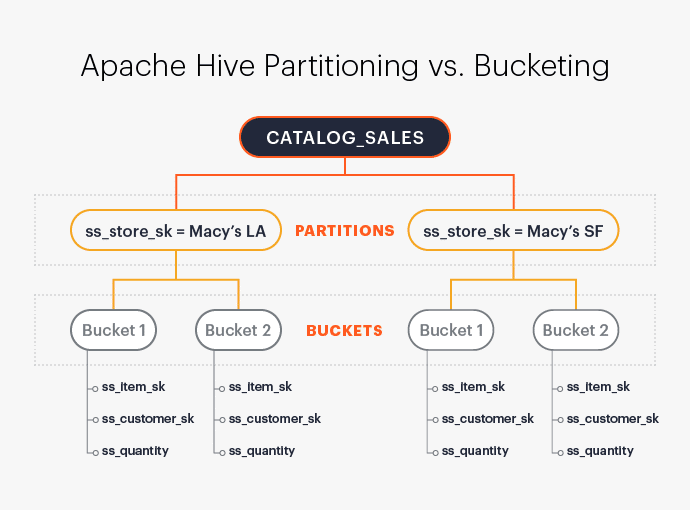
A table can have both partitions and bucketing info in it; in that case, the files within each partition will have bucketed files in it. For example, if the above example is modified to include partitioning on a column, and that results in 100 partitioned folders, each partition would have the same exact number of bucket files – 20 in this case – resulting in a total of 2,000 files across all partitions.
How to Implement Hive Bucketing with Okera
As of Okera’s 2.0 release, we now support Hive bucketing. (For specific details, you can refer to our documentation.)
For hash joins on two tables, the smaller table is broadcasted while the bigger table is streamed. When two non-bucketed big tables are joined, the broadcast table needs to fit into memory, which often creates out-of-memory errors due to memory constraints.
However, when these large tables are bucketed based on a common bucketing column, the joins are evaluated much more efficiently. The joins are now evaluated at the bucket level since we know now that the buckets match for both tables. Resource requirements are now considerably reduced, and the time to execute a query is decreased multifold.
Now let’s look at a specific example of bucketing in hive and how it can be used in Okera.
Bucketed vs. Non-Bucketed Query Performance
For this demonstration, we’ll use the standard tpc-ds tables. The big table samples will be catalog_sales, store_sales and store_returns. We’ll also use item, date_dim and store as small tables for query purposes. You can read more about the full schema used, along with the queries run, here on Github.
The chart below compares the same data accessed as bucketed vs non-bucketed table queries for three different variations. Those queries were chosen in such a way to demonstrate what a combination of big-medium, big-big table joins look like.
Primarily we have three datasets used for the queries,
catalog_sales – 164 GB, 143 Million rows (Big)
store_sales – 220 GB, 2.87 Billion rows (Big)
store_returns – 25 GB, 287 Million rows (Medium)
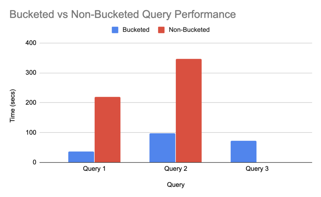
Query 1: Big-Medium tables join. This query has a join between the catalog_sales and store_returns tables.
Query 2: Join 2 Big-Medium tables. This query has a join of 2 joins. catalog_sales joined with store_returns and store_sales joined with store_returns.
Query 3: Two big tables join. This query has a join between the catalog_sales and store_sales tables. (Yes, the graphic looks unusual. No, this is not a mistake.)
In all cases, bucketed tables take less time to return than non-bucketed tables; 2-3x faster in the case of the first and second queries. In the case of the third query, the non-bucketed join results in `out of memory` for the given test resources.
For a traditional hash join on the non-bucketed tables, when joining the two big tables store_sales (220GB) and catalog_sales (164GB), the smaller one is broadcasted in each worker node in Okera to perform the join between each row of these tables. But since the catalog_sales table, while technically the “smaller” one, is still 164GB, it would not fit into the memory of the worker node used in this test which has a memory cap of 64 GB.
This problem is solved in the case of the bucketed table, where the join between the two tables happens only at the bucket level; for each bucket on the store_sales table, corresponding catalog_sales buckets are loaded for join comparison. This way, the memory utilization is kept very low.
Conclusion
As we just went through, bucketing in hive is very useful for certain big dataset joins which would otherwise not be possible without using up higher-end compute resource capacity. In addition, hive bucketing is more efficient for queries with filters on bucketing columns and aggregates.
Bucketing tables also can result in more efficient use of overall resources; memory utilization is low when the joins are done at the bucket level, instead of doing a full broadcast join of one of the tables. The greater the number of buckets, the less memory is needed – but too many buckets can create unneeded parallelism. It may take some experimenting at first, but eventually, you will figure out the ideal bucket count for highly efficient scans of the datasets.